
Target Audience for Direct Marketing in Starbucks Rewards Mobile App

Photo by Daiga Ellaby
This is the technical report I wrote for the capstone project in Udacity Data Science Nanodegree. The code for this project can be found on my GitHub here.
1. Project Definition
1.1. Project Overview
In this project I analyze the customer behavior in the Starbucks rewards mobile app.1 After signing up for the app, customers receive promotions every few days. The task is to identify which customers are influenced by promotional offers the most and what types of offers to send them in order to maximize the revenue.
There are three types of promotions:
- discount
- bogo (buy one, get one free)
- informational - product advertisement without any price off
Each offer is valid for certain number of days before it expires. Discounts and bogos have also different difficulty level, depending on how much the customer has to spend in order to earn the promotion. Promotions are distributed via different multiple channels (social, web, email, mobile).
All transactions made through the app are tracked automatically. The app also records information about which offers have been sent, which have been viewed and which have been completed and when these three events happened.
1.2. Dataset Overview
The data is organized in three files:
portfolio.json(10 offers x 6 fields) - offer types sent during 30-day test periodprofile.json(17000 users x 5 fields) - demographic profile of app userstranscript.json(306648 events x 4 fields) - event log on transactions, offers received, offers viewed, and offers completed
Here is the schema and explanation of each variable in the files:
portfolio.json
- id (string) - offer id
- offer_type (string) - type of offer ie BOGO, discount, informational
- difficulty (int) - minimum required spend to complete an offer
- reward (int) - reward given for completing an offer
- duration (int) - time for offer to be open, in days
- channels (list of strings)
profile.json
- age (int) - age of the customer
- became_member_on (int) - date when customer created an app account
- gender (str) - gender of the customer
- id (str) - customer id
- income (float) - customer’s income
transcript.json
- event (str) - record description (ie transaction, offer received, offer viewed, etc.)
- person (str) - customer id
- time (int) - time in hours since start of test. The data begins at time t=0
- value - (dict of strings) - either an offer id or transaction amount depending on the record
1.3. Problem Statement
The aim of this project is to identify target audience for a successful marketing campaign in direct marketing:
Direct marketing describes the marketer’s efforts to directly reach the customer through direct marketing communications (direct mail, e-mail, social media, and similar “personalized” or one-on-one means). The direct marketiing effort requires marketers to have a target list of customers that will each receive a marketing message tailored to their needs and interests. — John A. Davis: “Measuring Marketing”, 3d Edition, 2018, Part 8.
To solve this task, I performed customer segmentation using K-means clustering technique.
The idea is to divide app users into major groups - those more prone to discounts vs. those more keen on bogos vs. those that are not interested in promotions at all. The number of groups was decided at the later stage depending on the actual patterns in the final dataset.
1.4. Metrics
The critical decision in customer segmentation task is to choose the optimal number of segments. The problem with unsupervised machine learning is that it doesn’t have clearly defined benchmark metrics for model performance evaluation on par with supervised ML (e.g. accuracy score, f1-score, AUC, etc.). Instead there is a number of heuristics that aid analysts during decision-making process, but which ultimately don’t say anything whether the modeling results are good or bad. For k-means clustering, these heuristics are elbow curve method and silouhette score for deciding upon optimal number of clusters (see section 5.1. for more details).
To evaluate the segmentation results, I relied on the following marketing metrics2:
- Response Rate (RR) - the percentage of customers who viewed an offer relative to the number of customers that received the offer
- Conversion Rate (CVR) - the percentage of customers who completed an offer relative to the number of customers who viewed an offer
These two marketing metrics help marketers improve efficiency and reduce costs of a marketing campaign. The response rate tells how many customers are interested in offers, while the conversion rates show whether the offers sent were attractive enough to complete them.
By calculating each customer’s RR and CVR for all bogos, discounts and informational offers sent to him/her, I was able to evaluate the resulting segments in alignment with the project’s task, i.e. identify target audience for each offer type.
2. Data Munging
2.1. Data Cleaning
Similar to most data science tasks, the data cleaning and munging consumed the most amount of time when I worked on this project.
The first step was to combine the three datasets (portfolio, profile, transactions) into one final dataset. Because the project’s goal was to identify the customer segments based on their engagement with promotional offers, I decided to aggregate data at the level of each customer. However, before that was possible I needed to reorganize transactions data which was rather messy. In the following I describe the major challenge confronted here.
Correcting Offers Completed and Offers Viewed
The particular challenge with event log data was that it didn’t take into account the particular sequence of user’s interactions with offers. Thus, the app marked offers as completed when they satisfied offer criteria (expiration date and amount to be spent). This means that users might have earned rewards even when they didn’t view an offer. Similarly, the offers viewed didn’t take timing into consideration, which resulted into a situation when offer was counted as viewed even if a user viewed an offer after it expired. As a result, the completed and viewed offers as they were recorded in the event log didn’t reflect the actual campaign’s effect and the overall campaign results were distorted.
To address this problem, I identified which offers were viewed during the offer time window (before expiration date) and which offers were completed after viewing and before expiration date. These were separated from offers that were incorrectly attributed as completed or viewed. Both CVR and RR metrics reported here are based on the corrected values.
The technical side of this step can be summarized as follows.
Create unique identifier for each offer sent:
To evaluate which offers were viewed and completed correctly, I had to organize data at the offer level with timestamps for each event (received, viewed, completed). However, some customers received the same offer type more than once, meaning that the offer id is not a unique identifier in this case. When aggregating this data at later stage, information on these offers will be lost unless we create unique identifiers for them. To get an idea, there are 76277 offers sent, out of which 51570 offers were sent to a certain customer only once, while 24707 offers of the same types were sent more than once.
So I created a unique identfier for each offer by combining groupby() and cumcount() functions to count how many times the same offer type was sent to the same person and then combine this counter with the offer id into a unique identifier:
#create unique identifier for each offer sent (because same offers could be sent more than once)
  starbucks_time['id_unique_received'] = starbucks_time[starbucks_time.offer_received == 1].groupby(['person', 'offer_id']).cumcount()
  starbucks_time['id_unique_viewed'] = starbucks_time[starbucks_time.offer_viewed == 1].groupby(['person', 'offer_id']).cumcount()
  starbucks_time['id_unique_completed'] = starbucks_time[starbucks_time.offer_completed == 1].groupby(['person', 'offer_id']).cumcount()
  starbucks_time['id_unique_events'] = starbucks_time[['id_unique_received', 'id_unique_viewed', 'id_unique_completed']].max(axis=1).values
  starbucks_time['id_unique'] = starbucks_time['offer_id'] + "-" + starbucks_time['id_unique_events'].apply(lambda x: str(x))
For instance, if the offer type 'fafdcd668e3743c1bb461111dcafc2a4' was sent to the same person twice, the first offer sent gets unique id as 'fafdcd668e3743c1bb461111dcafc2a4-0.0' while the second offer of the same type gets unique id of 'fafdcd668e3743c1bb461111dcafc2a4-1.0'.
Pivot timestamps data from long to wide format
Since the data in transactions dataset was in the long format, the next challenge was to organize it into wide format with combination of groupby(), max() and unstack() functions.
  # create columns with time for each event
  starbucks_time['offer_received_time'] = starbucks_time['offer_received']*starbucks_time.time
  starbucks_time['offer_viewed_time'] = starbucks_time['offer_viewed']*starbucks_time.time
  starbucks_time['offer_completed_time'] = starbucks_time['offer_completed']*starbucks_time.time
  starbucks_time = starbucks_time[['person', 'id_unique', 'offer_id', 'time', 'offer_received_time', 'offer_viewed_time', 'offer_completed_time']]

  # unstack values to get to the level of each (person, offer id) tuple
  # need to take max values to avoid 0s
  starbucks_time_full = starbucks_time.groupby(by=['person', 'id_unique', 'time']).max().unstack()
  starbucks_time_full.fillna(0, inplace=True)

  # create the final time-based dataset for each offer sent
  offers = pd.DataFrame(starbucks_time_full.index.get_level_values('id_unique'), starbucks_time_full.index.get_level_values('person')).reset_index()
  offers['offer_received_time'] = starbucks_time_full['offer_received_time'].values.max(axis=1)
  offers['offer_viewed_time'] = starbucks_time_full['offer_viewed_time'].values.max(axis=1)
  offers['offer_completed_time'] = starbucks_time_full['offer_completed_time'].values.max(axis=1)
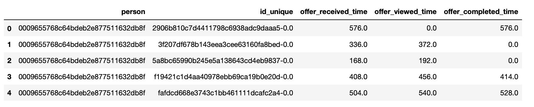
So from this:
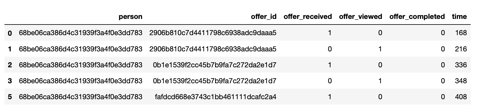
… we got to this:
Add offer end time
Then I combined the time-based data with portfolio data to access the duration of each offer and calculated the offer expiration timestamp by adding the duration time (converted from days to hours) to received timestamp in hours.
# add information about each offer from portfolio
  offers['id'] = offers.id_unique.apply(lambda x: x.split("-")[0])
  offers = offers.merge(portfolio, on='id', how='left')

  # add offer end time (convert duration time that is in days to hours)
  offers['offer_end_time'] = offers['offer_received_time']+offers['duration'].values*24
Identify completed offers and viewed offers correctly
Now I had all the needed information on offer level to correctly attribute offers as completed or viewed.
For offer to be counted as “viewed” it had to be viewed before offer expiration date.
offers['viewed_binary'] = offers.offer_viewed_time.apply(lambda x: 1 if x > 0 else 0)
offers['viewed_on_time'] = (offers.offer_viewed_time < offers.offer_end_time)*offers['viewed_binary']
For offer to be “completed” it had to meet these conditions:
- be completed before offer expiration date
- completed after viewing
offers['completed_binary'] = offers.offer_completed_time.apply(lambda x: 1 if x > 0 else 0)
offers['completed_on_time'] = (offers.offer_completed_time < offers.offer_end_time)*offers['completed_binary']

completed_before_expires = (offers.offer_completed_time < offers.offer_end_time)
completed_after_viewing =(offers.offer_completed_time > offers.offer_viewed_time)*offers['viewed_binary']
offers['completed_after_viewing'] = (completed_after_viewing & completed_before_expires)*offers['completed_binary']
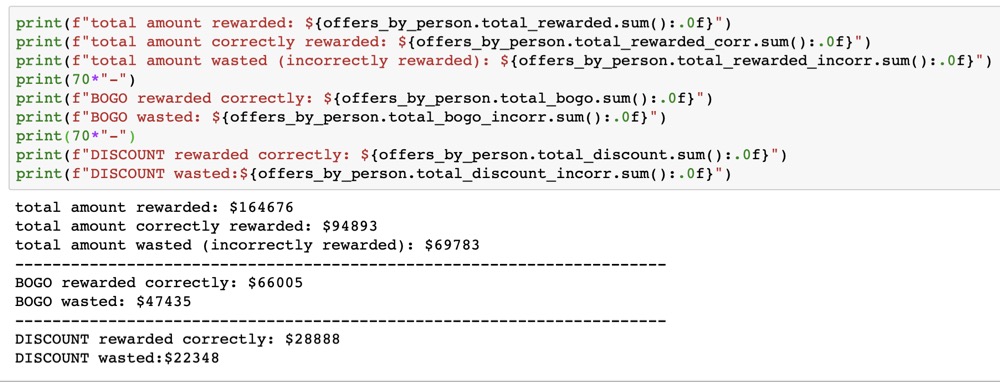
The effect of this “cleanup” is not to be underestimated. According to my analysis, Starbucks could have saved almost $70,000 if it tracked completed offers correctly:
2.2. Feature Engineering
The final dataset has 32 features, most of which were calculated or engineered. Thus, I created the following features:
total_amount(int): the amount spent by each customer during the 30 day test periodtotal_rewarded(int): the amount each customer was rewarded (Note: not the recorded sum, but correctly attributed sum)transactions_num(int): number of transactions each customer made during the test periodoffers_received(int): total number of offers received by each customeroffers_viewed(int): total number of offers viewed by each customeroffers_completed(int): total number of offers completed by each customerbogo_received,bogo_viewed,bogo_completed(int): the number of bogo offers correspondingly received, viewed and completeddiscount_received,discount_viewed,discount_completed(int): the number of discount offers correspondingly received, viewed and completedinformational_received,informational_viewed(int): the number of informational offers correspondingly received and viewedtotal_bogo,total_discount(int): the amount each customer got rewarded correspondingly on bogo and discount offersavg_order_size(int): average order size as total amount divided by number of transactionsavg_reward_size(int): average reward size as total amount rewarded divided by the number of discounts and bogo offers completedavg_bogo_size,avg_discount_size(int): average bogo size as the number of total bogo amount rewarded divided by total number of bogo completed and the corresponding numbers for average discount size for each customeroffers_rr,bogo_rr,discount_rr,informational_rr(int): response rates of each customer at the overall offer level, bogo, discount and informational leveloffers_cvr,bogo_cvr,discount_cvr(int): conversion rates of each customer at the general offer level and at the bogo and discount levels.
Note: All features that have to deal with offer viewing or completing reflect not recorded number, but correctly attributed number and the amounts that are based on these numbers reflect the correctly attributed sums, not the recorded sums (see 2.1. for more information). This ensures that we measure customer interaction with offers correctly.
2.3. Imputing Missing Values
It turned out that there are about 2175 customers (12.8%) with missing values in the profile dataset. Rows with missing data had no information on customer’s age, income and gender simultaneously. I implemented two strategies to deal with missing data in a function:
- drop the missing values all together (which is worse, since 12% is a lot of data)
- impute with median values for numerical columns (age and income) or impute the mode for categorical column (gender). The median values for age and income turned out to be 55 years and $64000 correspondingly and Male as the most frequent value for gender.
3. Analysis
3.1. Data Exploration
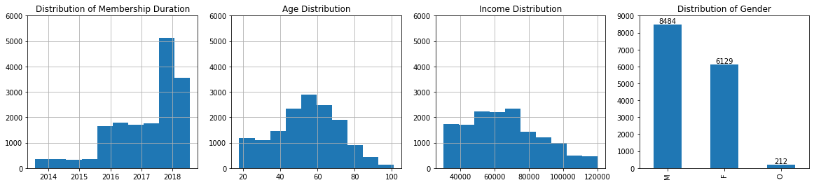
Customers: The typical Stabucks mobile app customer is middle-aged (median - 55 years) and has income of about $64000). During the experiment, the customers spent on average $104.44 (min - $0, max - $1608.7) and got $5.6 (min - $0, max - $55) rewarded. Furthermore, customers would make on average 8 transactions with the average order size being $13.34.
Offers: Customers would receive on average 4-5 offers, view about 3 offers and complete about 1 offer. The average return on bogo offers is higher than on discount offers - $3.8 vs $1.7. Each customer viewed on average 73% of offers he/she received (Response Rate), with bogo offers being viewed more often (73%) than discounts (61%) or informational offers (39%). Each customer reacted upon (CVR) about 34% of offers he/she viewed, with CVR for discounts being higher (38%) than for bogo (29%).
Customer-Offer Interactions: The original datasets contain information on 17000 customers, all with unique anonymized ids. During data exploration phase, it turned out that 16994 customers received offers, while 6 did not. Out of those who received, 16735 customers viewed offers, while 259 did not. Out of those who received & viewed, 10640 customers completed the offers, while 6095 did not. As a result, Viewing Rate is quite high - 98.4%, while the overall completion rate is much lower - 62.6%.
3.2. Data Visualization
Customer Profile
Number of Events: Received, Viewed, Completed
As noted in section 2.1., I reevaluated the number of events after imposing certain conditions. One can see from the plot below that the actual viewing and completion rate is much less:
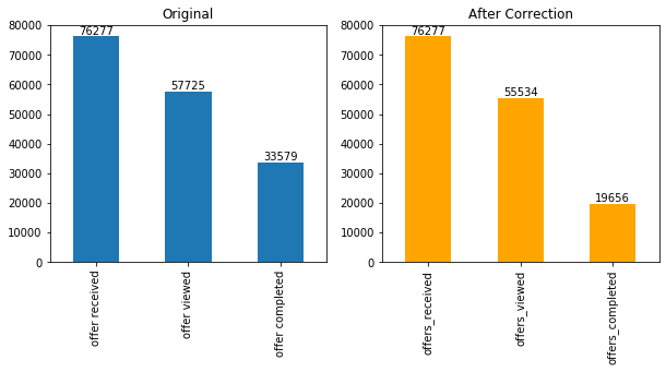
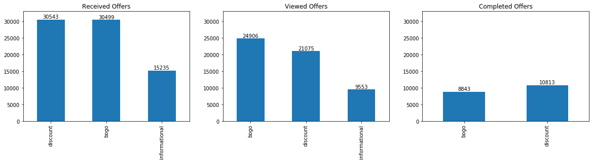
By offer type these corrected values look like this:
I also calculated correlations of certain numerical features with the metrics of interest:
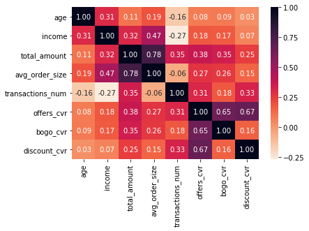
From the correlation matrix, it seems like not the profile features, but rather spending habits (like number of transactions and total amount) seem to correlate more with the conversion rates. For bogo_cvr total amount spent seems to be more defining, while for discount_cvr - transaction frequency.
4. Data Preprocessing
The linear unsupervised machine learning and K-means clustering in particular rely on distances as measure of similarity and hence are prone to data scaling. To account for this problem, I further transformed the data before clustering - one-hot encoded categorical features, scaled the features and perform dimensionality reduction.
4.1. One Hot Encoding
The majority of features in the final dataset are numerical except for gender, which is categorical. This column had to be one-hot encoded, meaning its values had to be converted into binary (dummy) variables that take on either 0 or 1 . Earlier in the project I also one-hot encoded offer types.
Besides that I decided to transform the original became_member_on into categorical column with membership years as its values. The categorical membership column now could serve as a proxy for customers loyalty and was easier to interpret afterwards. Because there are only 6 possible years (2013-2018), the one-hot encoding of this feature didn’t increase the data dimensionality that much.
4.2. Feature Scaling
Next, the data was transformed to achieve the same scale needed for PCA and K-means clustering. This is an important step, as otherwise features with large scale would dominate the clustering process. I implemented two popular scaling techniques available in scikit-learn library (but found that standardization produced better results - see more in 4.5.)):
StandardScaler: standardizes/normalizes the data by substracting the mean and dividing by the standard deviation;MinMaxScaler: transforms the data so that all of its values are between zero and one.
4.3. Dimensionality Reduction with PCA
Dimensionality reduction helps reduce the noise in the data by projecting it from high-dimensional into low-dimensional space, while retaining as much of the variation as possible. The ML algorithms thus can identify patterns in the data more effectively (because of less variability in data) and more efficiently (because of less dimensions hence less computational power needed to make calculations).3
In this project, I used standard Principal Component Analysis (PCA). In the first step, I performed PCA on the original number of dimensions (i.e. features) and visualized the importance of each component with the scree plot:
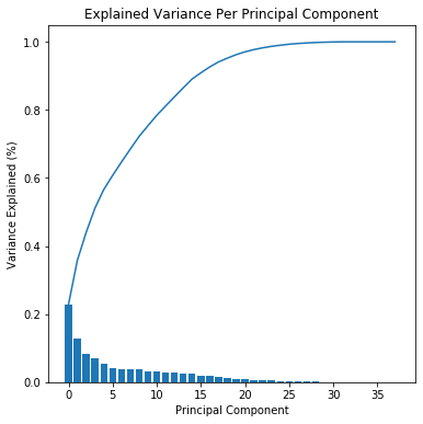
As a good rule of thumb, one should keep as many components that together explain about 80% of variance. From the scree plot, one can see that the first 10 components in total capture almost 80% of the variance in the data. I wrote the code to automatically select this number of PCA components, so that I could easily test different datasets when clustering:
pca = PCA()
X_pca = pca.fit_transform(starbucks_scaled)
cum_expl_var_ratio = np.cumsum(pca.explained_variance_ratio_)

#choose number of components that explain ~80% of variance
components_num = len(cum_expl_var_ratio[cum_expl_var_ratio <= 0.805])
print(f"number of pca components that explain 80%: {components_num}")
pca = PCA(components_num).fit(starbucks_scaled)
starbucks_pca = pca.transform(starbucks_scaled)
5. Model Implementation
5.1. K-means clustering
The goal of clustering is to identify groups of data, in which values are similar to each other. K-means is a popular algorithm in that it finds the data points that are closest to the cluster centroid. In technical terms, it tries to minimize the intra-cluster variation measured as the sum of the squared distances of each data point to the mean of the assigned cluster. 4
Since the cluster means are assigned initially randomly, there is no guarantee that it will produce the optimal clustering result. It is usually recommended to run k-means algrorithm several times. Therefore, I set the number of iterations to 10.
# Over a number of different cluster counts...
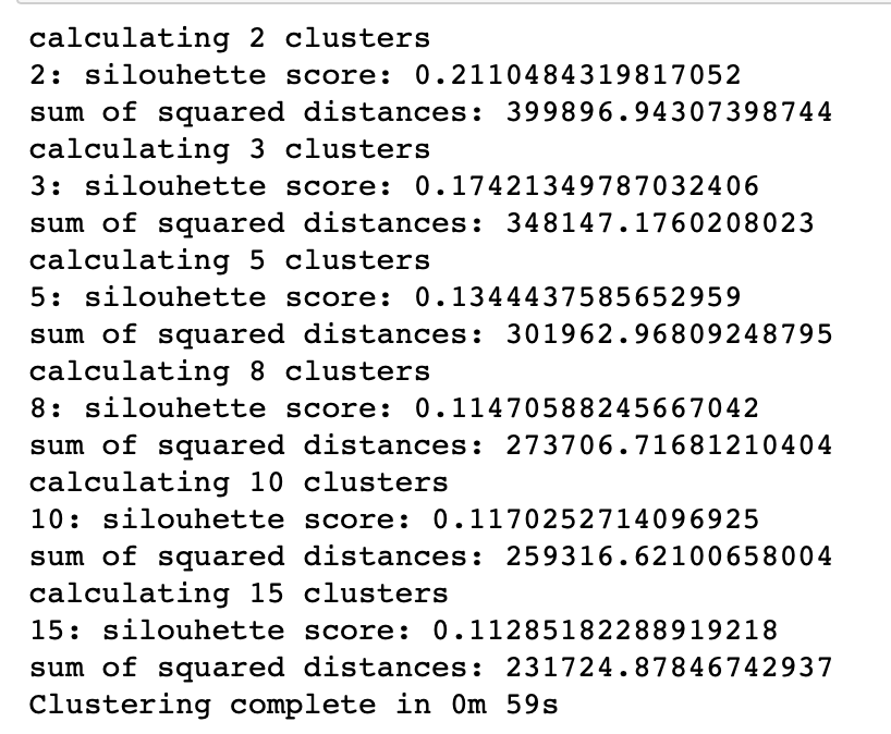
range_n_clusters = [2, 3, 5, 8, 10, 15]
sum_of_squared_distances = []
since = time.time()
for n_clusters in range_n_clusters:
cluster_start = time.time()
print("calculating {} clusters".format(n_clusters))
# run k-means clustering on the data and...
clusterer = KMeans(n_clusters=n_clusters, n_init=10).fit(starbucks_pca)
print(f"{n_clusters}: silouhette score: {metrics.silhouette_score(starbucks_pca, clusterer.labels_, metric='euclidean')}")
# ... compute the average within-cluster distances.
sum_of_squared_distances.append(clusterer.inertia_)
print("sum of squared distances:", clusterer.inertia_)
#print("time for this cluster:", time.time() - cluster_start)
time_elapsed = time.time() - since
print('Clustering complete in {:.0f}m {:.0f}s'.format(time_elapsed // 60, time_elapsed % 60))
When deciding upon the optimal clusters number, I relied on two heuristics - the elbow curve and silhouette score. The elbow curve plots the within-cluster sum of squared distances (WSS) as a function of number of clusters. As the number of clusters increase, there will be less and less data points in each cluster and hence they will be closer to their respective centroids, dropping WSS. One should choose a number of clusters so that adding another cluster doesn’t improve much better the total WSS. On the elbow curve, this will look like an elbow shape, hence the name.
Because elbow method is sometimes ambiguous, I used the average silouhette method to assist in deciding upon cluster number. The silhouette value is a measure of how similar an object is to its own cluster (cohesion) compared to other clusters (separation). The average silhouette method then computes the average silhouette value for all data points, which can range from -1 to +1 with values closer to 0 meaning the clusters overlap. The higher the score, the better the points in the cluster match their own cluster and worse the neighboring clusters.
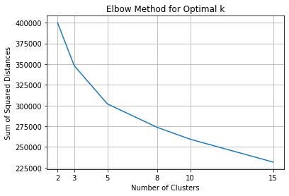
From the elbow curve plot above, we see two potentially good cluster numbers - 3 and 5. Because the silhouette score is higher for 3 clusters than for 5 clusters and after checking the results visually I decided to keep 3 clusters. The 3 clusters are also aligned with the metrics better, as the clusters are formed around the offer types - bogo, discount and neither.
In general, however, the silhoutte scores are not particularly high - around 0.17, meaning that the clusters overlap and there is no clear separation. This is usual in marketing problems, where the boundaries between segments based on some people traits or behavior are rather vague. To see if there are any other better solutions, I tested different number of clusters along with other analytical steps discussed in the next section.
5.2. Refinement
When going through the full analytical cycle for the first time, I made the following decisions that predetermined the clustering results:
- the decision to impute values
- the decision to use standardization when scaling
- the decision to perform PCA
- the decision to create 3 clusters
In an attempt to diminish the influence of these decisions, I decided to refactor the code in form of functions that would allow quick experimentation. In particular, I was keen on checking the clustering results when:
- missing values were dropped instead of imputed
- MinMax scaler was used instead of Standard Scaler
- no PCA was performed
- different number of clusters were specified
6. Results
6.1. Model Evaluation
To interpret clustering results, I first inversed the values that resulted from using Scaler and PCA:
def interpret_cluster(cluster_num, df, minmax):
    '''
    Performs inversing the results of PCA and Scaler to allow cluster interpretation
    Input:
        cluster_num: number of clusters that were used to perform clustering
        df: data frame used for clustering
        minmax (bool): condition whetherminmax scaler was used
    Output:
        results_df: data frame with inversed values for one cluster
    '''
    pca_inversed = pca.inverse_transform(clusterer.cluster_centers_[cluster_num, :])

    if minmax == True:
        scaler_inversed = np.around(scaler.inverse_transform(pca_inversed.reshape(1, -1)), decimals=2)
        results_df = pd.DataFrame(scaler_inversed.ravel(), df.columns)
    else:
        scaler_inversed = np.around(scaler.inverse_transform(pca_inversed), decimals=2)
        results_df = pd.DataFrame(scaler_inversed, df.columns)

    return results_df
With the help of another function, I created the final clustering results data frame and plotted its results against mean values (red line) for each feature:
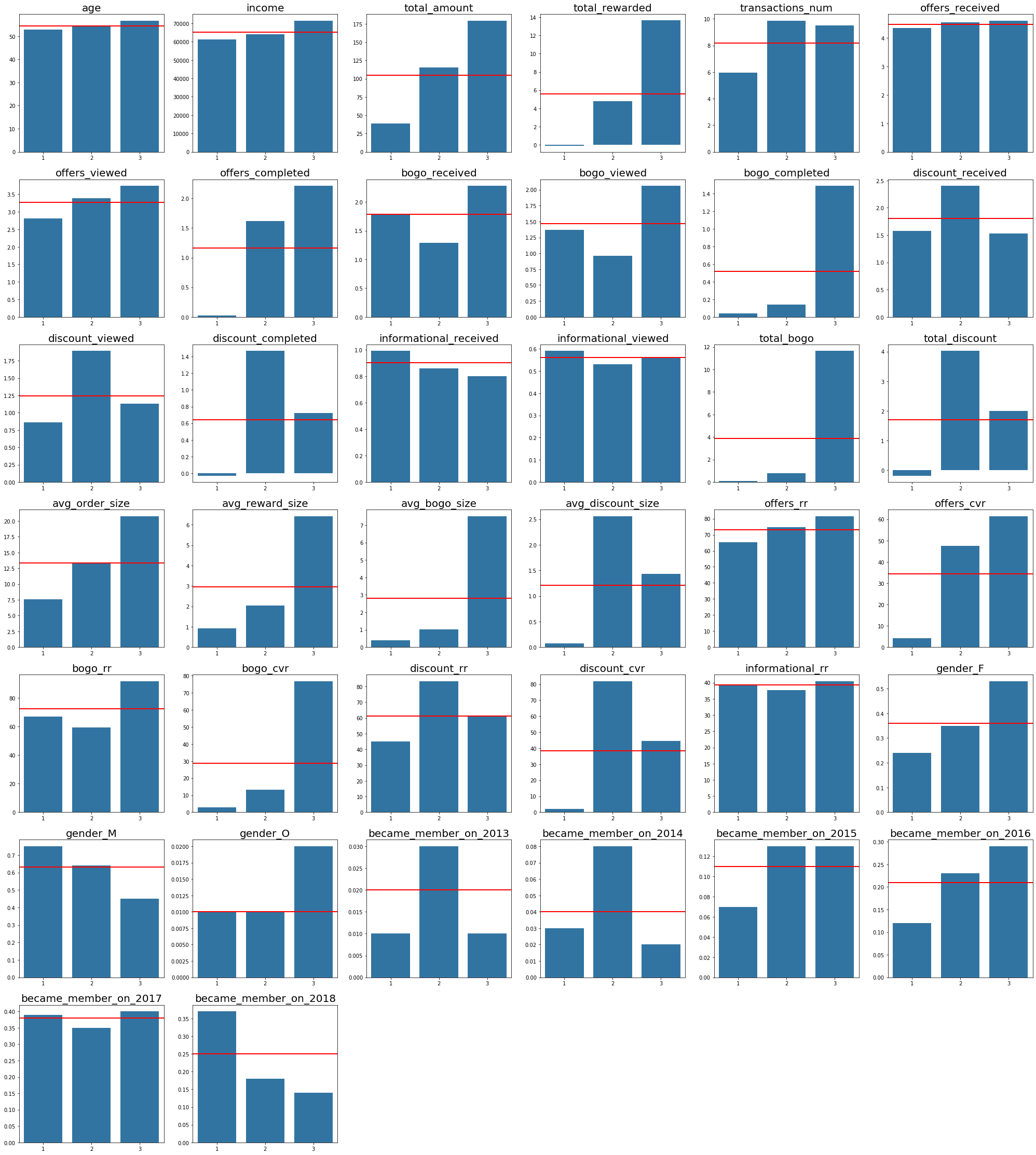
Based on the above plots, I came to this clustering results:
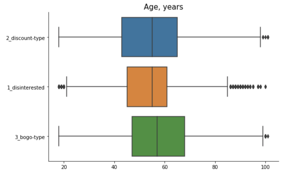
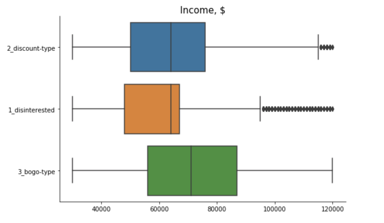
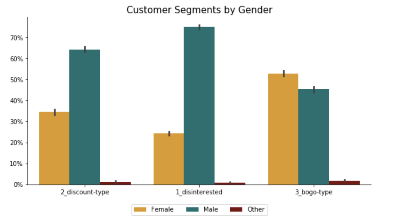
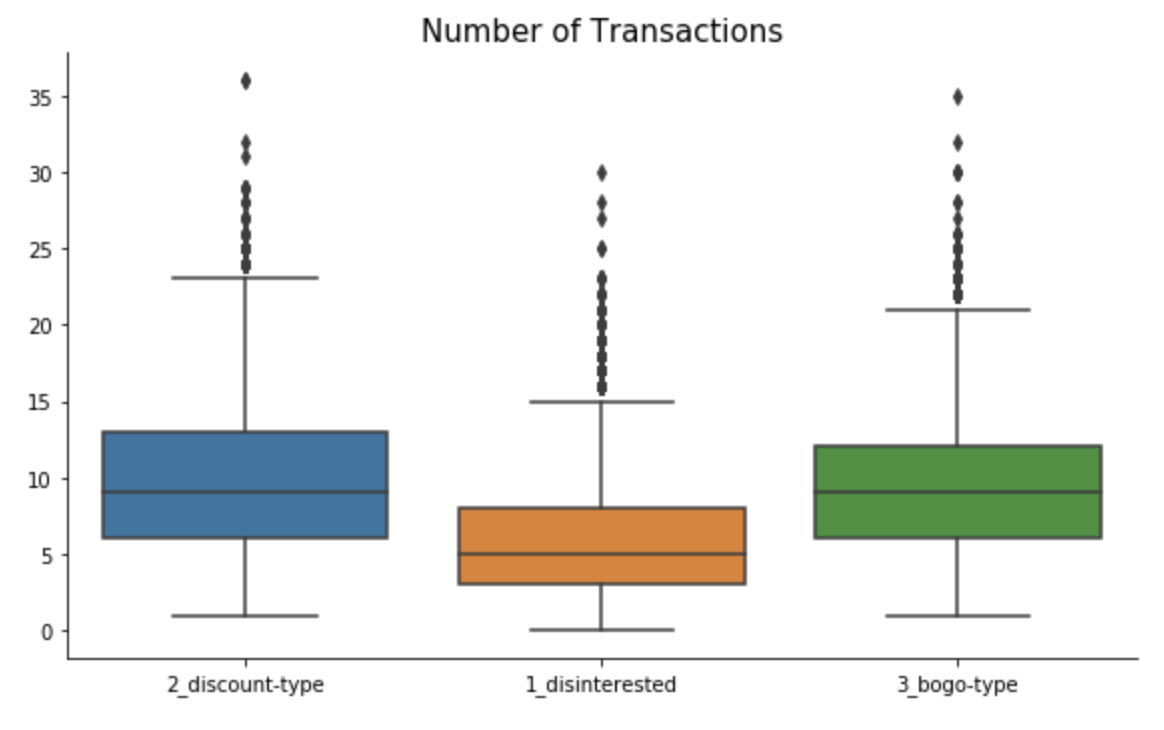
Cluster 1 - “Disinterested”: This group of customers are predominantly male that just recently became members. They tend to spend not much with below average number of transactions and small average order size. Although slightly more than 60% in this group view offers, they don’t complete them.
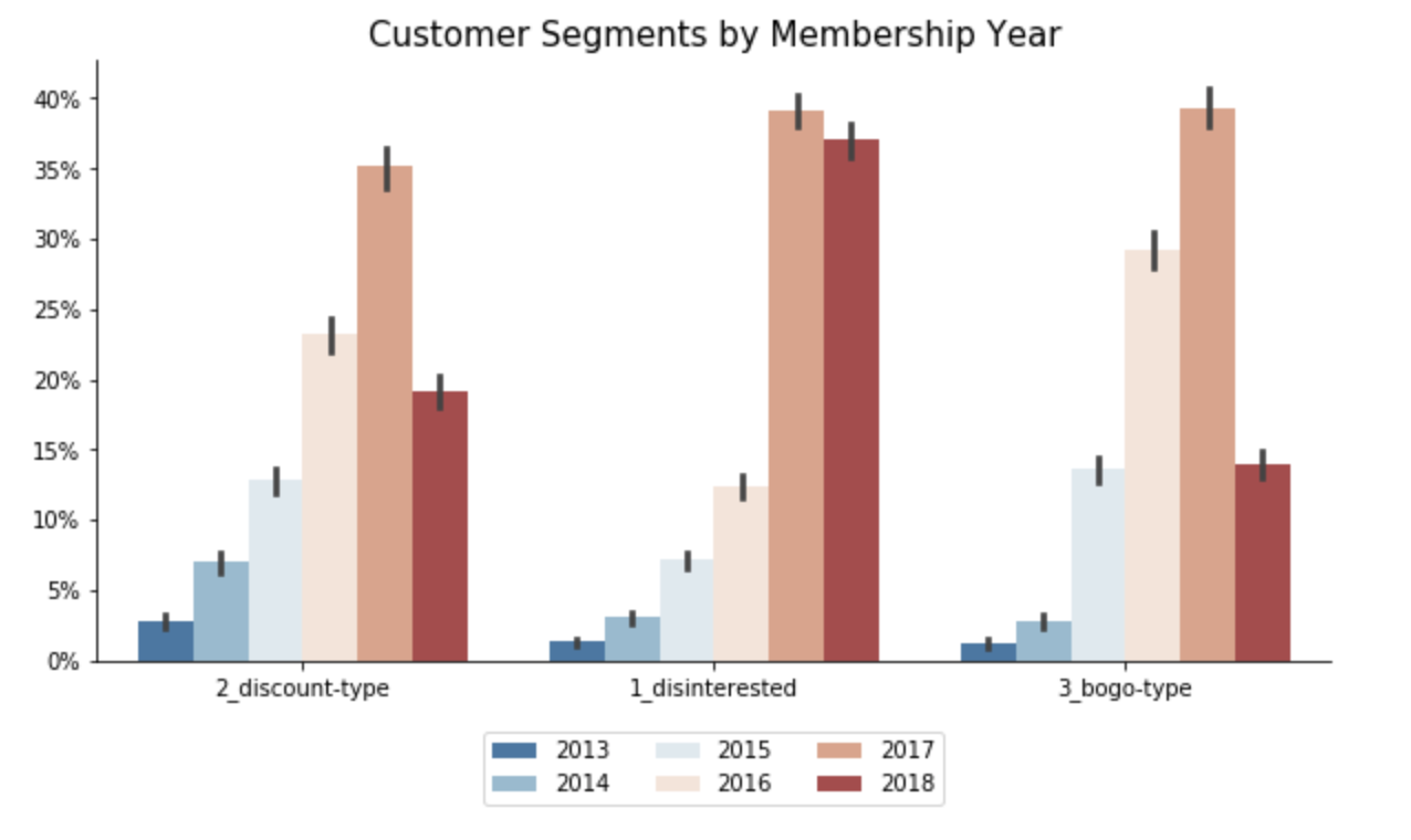
Cluster 2 - “Discount-Type”: This group of customers are also mostly male but with the longest membership status (since 2013/2014). They tend to receive more discounts, which they love and actively complete. Their spending habits are slightly above average - they make small orders, but buy frequently.
Cluster 3 - “Bogo-Type”: This is the only segment where female dominate over male. The customers in this group tend to be older and have higher income. They are loyal customers for few years already. They spend a lot - make huge orders and buy frequently. With such spending habits, no wonder that they are intersted in bogo and get rewarded the most. They complete bogo offers way beyond average, but also react to discounts from time to time.
6.2. Validation
Since clustering techniques don’t have good metrics like supervised modeling to evaluate the modeling results, I relied on results validation through visualization of segments.
Here are the plots with the final results:
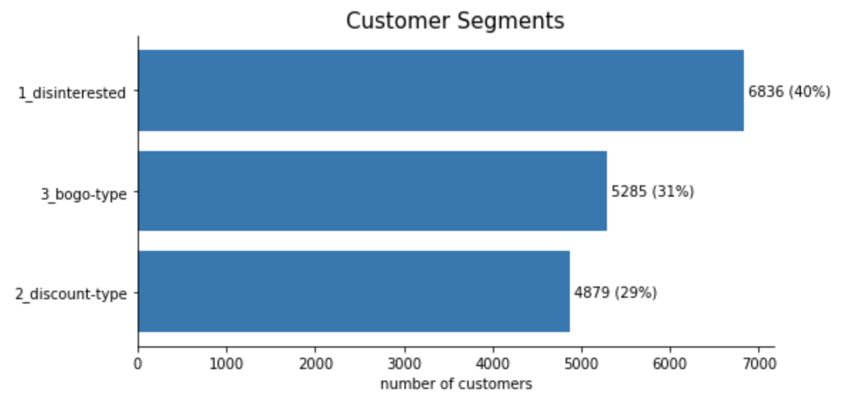
Segments Size
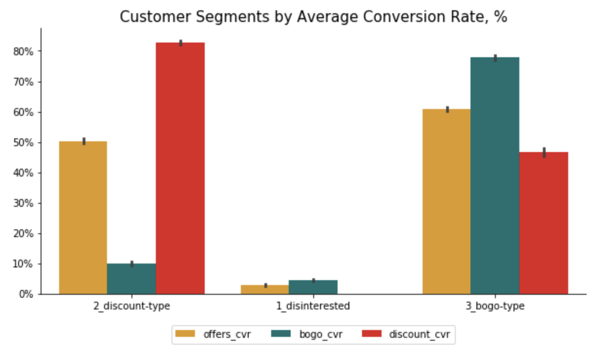
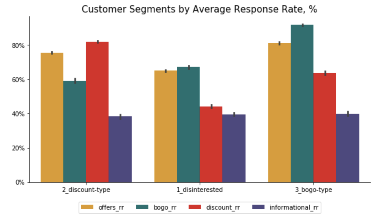
Metrics
Profile
Spending Habits

6.3. Justification
As noted in section 4.5, I tested several clustering versions - with MinMax/Standard Scaler, with/without PCA and on dataset with smaller features. In general, clustering with MinMax Scaler had different results from Standard Scaler, which were not really aligned with the metrics (i.e. differentiated between bogo/discount type worse). This is probably because I have a big number of numerical features with different scales, while MinMax works better for cases where the distribution is not Gaussian (e.g. categorical features).
In all other cases, the clustering results were good and differed mainly in the cluster sizes. As a result, I conclude that the initial decision to use Standard Scaler and perform PCA was correct.
7. Conclusion
7.1. Reflection
Having segmented data into 3 segments, we now have better insight into Starbucks rewards user base. The clustering results would allow the company to better target audience with tailored offers in the next marketing campaign.
To arrive at this solution, I performed the full analysis cycle - cleaning and preprocessing the data, dealing with missing values, feature engineering, feature scaling, one hot encoding, dimensionality reduction and clustering. I also wrote a number of functions to generate the clustering results automatically, which allowed some quick experimentation.
While working on this project, I found that data preprocessing consumed a lot of time and was particularly challenging in this case because the event log didn’t account for particular marketing needs. As a marketer, for instance, I would not like when my response rates would be contaminated by offers viewed after the offer expiration date. Similarly, I would not like to waste marketing budget on customers that would buy the product even without promotional offer or earn rewards even when not viewing the offers. By imposing conditions on when offers should be considered as properly “viewed” or “completed”, I managed to fix this problem with original records. In the future, however, it would be advisable for Starbucks to implement a different tracking strategy as, for instance, by putting a reference code in the campaign message and asking the consumers to mention the code in order to receive the reward.
7.2. Improvement
One of the possible ways to improve the clustering results is to predict the missing age, income and gender values instead of simply imputing them. In this case, I would use the supervised machine learning, experimenting with different models like RandomForest, AdaBoost, etc. Another useful improvement would be to use the clustering results as labels in supervised modeling to actually predict customer’s probability of completing the offer. This would be a nice practical application that would allow extension on new customers and so would assist in executing a successful marketing campaign in the future.
-
The data is simulated but mimics the actual customer behavior closely. It is also a simplified version, since it contains information only about one product, while the real app sells a variaty of products. Finally, the data provided contains information on transactions/offer events during the 30 days trial test. ↩
-
Farris, P., Bendle, N., Pfeifer, Ph., Reibstein, D. (2016): Marketing Metrics: The Manager’s Guide to Measuring Marketing Performance, 3rd Edition. Pearson Education, Inc. Chapter 8 “Promotions”, pp. 271-293. ↩
-
cf. Ankur A. Patel (2019): “Hands-On Unsupervised Learning Using Python”. ↩
-
cf. Peter Bruce, Andrew Bruce (2018): “Practical Statistics for Data Scientists”, O’Reilly. ↩

Leave a comment